
The Gini coefficient is a standard measure of inequality that summarises how unevenly income or wealth is distributed within a country. It ranges from 0 to 1, where 0 represents perfect equality — everyone has exactly the same income — and 1 represents perfect inequality, where a single person holds all income and everyone else has none.
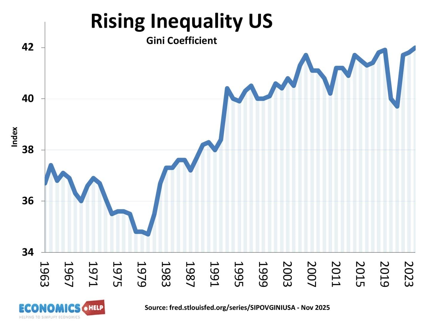
Gini coefficient for the United States, this shows that income inequality has increased since 1980.
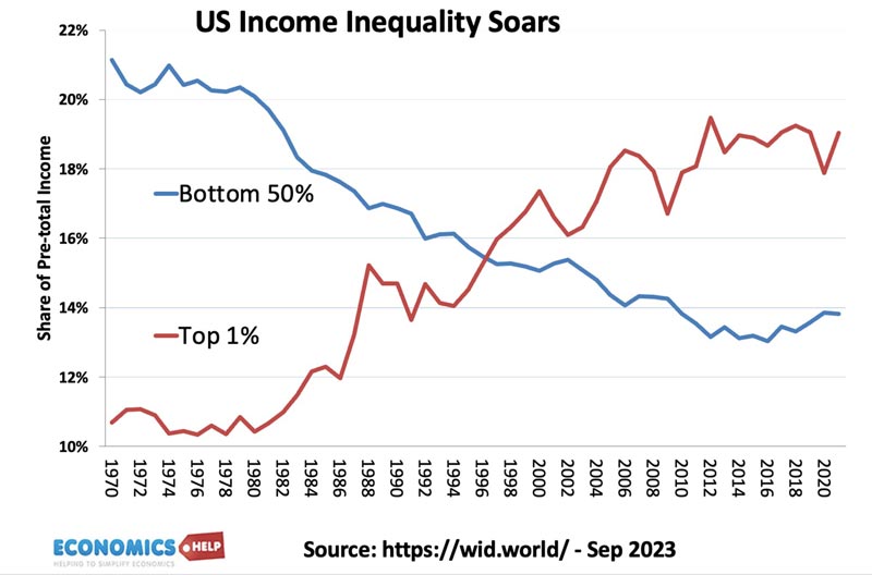
Another way of visualising this inequality is showing income share of top 1% and top 50%. The top 1% have increased income share, the bottom 50% have seen a fall.
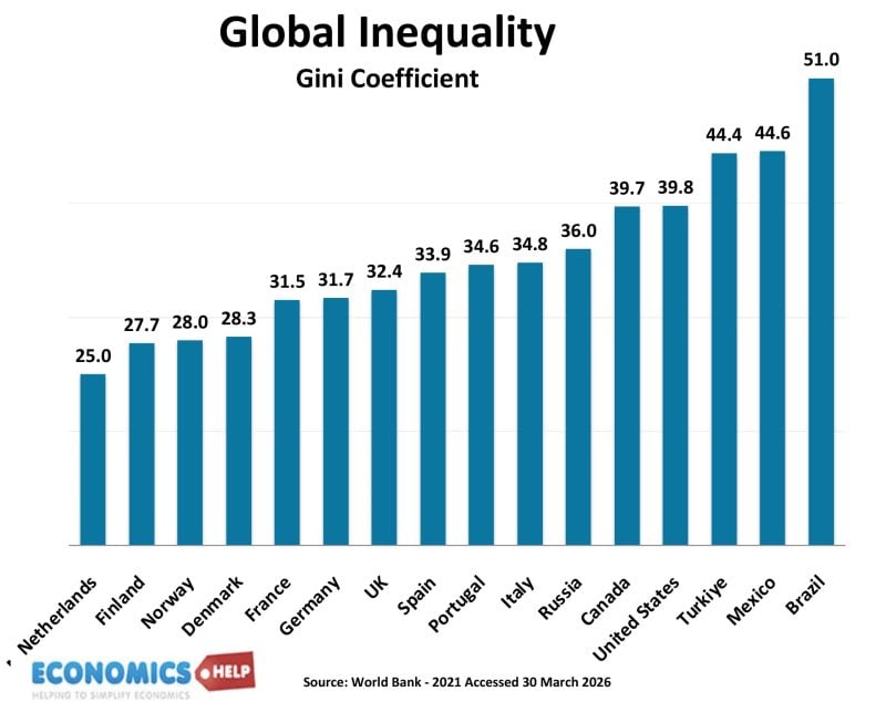
In practice, advanced economies’ Gini usually fall between about 0.25 and 0.45 for disposable-income inequality, while countries with weaker tax and welfare systems tend to sit higher.
Gini Coefficient and Lorenz Curve
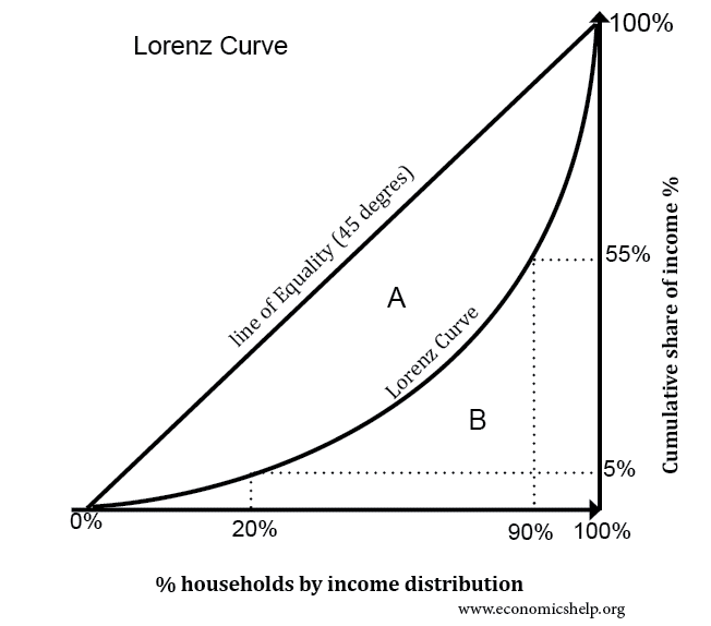
The Gini is derived from the Lorenz curve, which plots the cumulative share of income against the cumulative share of the population. The more the Lorenz curve bends away from the 45-degree line of perfect equality, the larger the Gini becomes.
The formula for gini coefficient is

In this example, the second Lorenz curve is closer to line of equality, so area A becomes a smaller share of the total area (A+B).
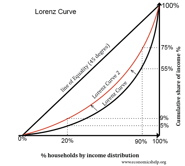
Therefore, the gini coefficient falls, indicating greater income equality.
Limitations of Gini Coefficient
- The gini coefficient shows overall income inequality; however, it is limited for example, there could be a shift in income inequality with the top 0.1% gaining a bigger share, but the overall area A is the same. The Gini coefficient suggests nothing has changed but actually, inequality is now more extreme at the top.
- Because it is based on relative differences, the Gini does not show whether living standards are rising or falling in absolute terms; a society can have a stable Gini while poverty worsens.
- It reacts slowly to changes at the very top because the Lorenz curve compresses the upper tail of the distribution, making extreme top-1% or top-0.1% inequality hard to see
- The Gini index can be affected by data quality — especially under-reporting of income, tax avoidance, or missing top incomes — and it cannot capture non-income dimensions of inequality such as wealth, health, education, or regional gaps. This is often an issue with the rich having offshore wealth and hidden income.
What determines Gini Coefficient?
Examples of Gini Coefficient
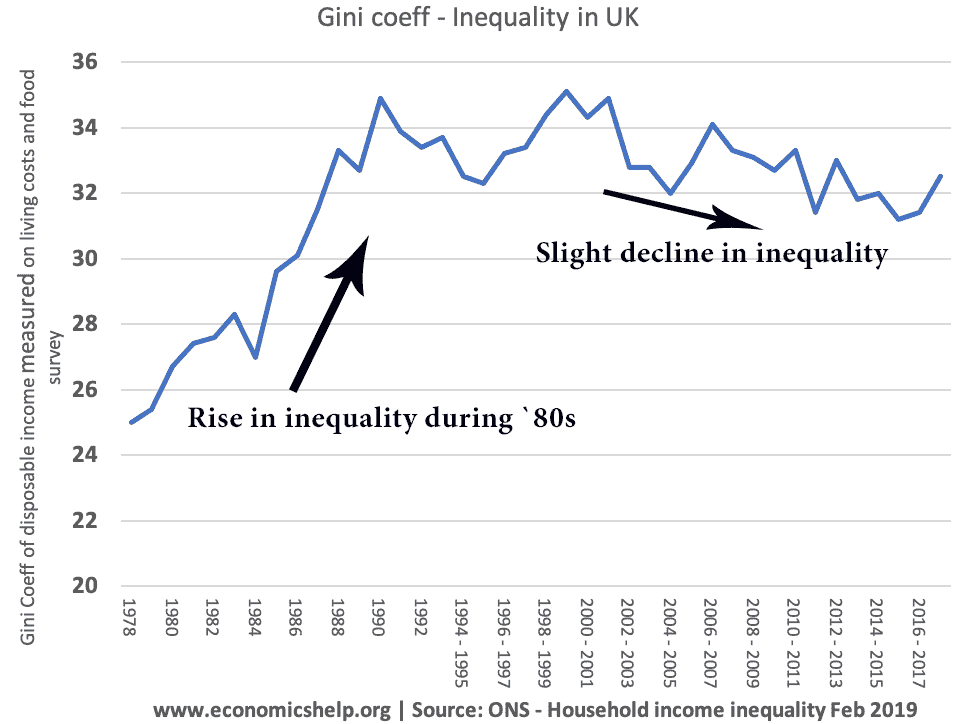
In the 1980s, the UK had a rise in the gini coefficient. This was due to

- Decline in manufacturing, and manufacturing jobs
- Rise in unemployment, which led to lower income for those out of work
- Tax cuts for high income earners
- Growth of financialization and high paying income inequality
- Rising wealth, which helps those with assets get extra income from assets.

This shows changes in inequality. One trend is how US inequality increased from the 1980s
More detail on why income inequality increased in the US
Related
Sorted-income Gini Formula
The sorted-income formula is the most practical way to calculate the Gini coefficient when you have a list of individual incomes. First, sort the incomes from lowest to highest. Then use this formula:

where:
• xᵢ is the income of the i-th person in the sorted list
• n is the number of people
• i runs from 1 (poorest) to n (richest)
The first term, 2 Σ (i · xᵢ) / (n Σ xᵢ), gives more weight to higher incomes because they appear later in the sorted list. The second term, (n + 1) / n, adjusts the scale so the result is between 0 and 1.
Complex Gini Formula

It looks complex, but the idea is simple. The top part adds up the absolute income differences between every pair of people in the population. If everyone has the same income, all these differences are zero and the Gini becomes zero. If incomes vary a lot, these pairwise gaps become large and the Gini rises.
The denominator, 2 n² μ, is just a normalising factor so the final result lies between 0 and 1. n² is the number of pairwise comparisons, μ is the average income, and the 2 removes double-counting (because the difference between person A and B is the same as between B and A).
This formula shows that the Gini coefficient is essentially the average income gap between all individuals, expressed relative to the mean income.
Although it is conceptually the clearest definition, it is:
- computationally heavy for large datasets (millions of pairwise comparisons)
- redundant because simpler formulas (like the sorted-income formula) give identical results much faster
About The Author
