The market supply curve shows the combined quantity supplied of goods at different prices.
The market supply curve is the horizontal sum of all individual supply curves.
Linear Supply curve
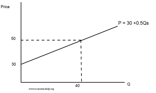
A linear supply curve can be plotted using a simple equation P
= a + bS
a = plots the starting point of the supply curve on the Y-axis intercept.
b = slope of the supply curve.
P = 30+0.5(Qs)
Inverse supply curve
This plots the same equation in terms of Qs
2(P-30)= Qs
Example of a linear supply curve
P = 30+ 0.5(QS)

| Q | P |
| 0 | 30 |
| 10 | 35 |
| 20 | 40 |
| 30 | 45 |
| 40 | 50 |
| 50 | 55 |
| 60 | 70 |
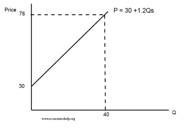
Shift in the slope of the supply curve
P = 30+ 1.2(QS)

P=30+1.2(Qs)
| Q | P |
| 0 | 30 |
| 10 | 42 |
| 20 | 54 |
| 30 | 66 |
| 40 | 78 |
| 50 | 90 |
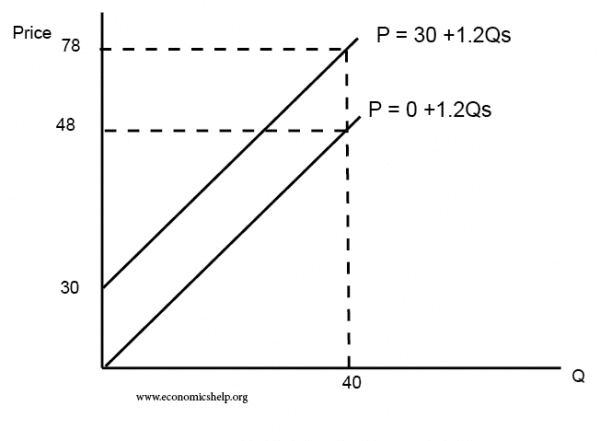
Shift in a – Shift in the supply curve

P = 0 + 1.2 (Qs) shifts the supply curve downwards so it starts at the 0,0.
Why is supply curve generally upward sloping?
Generally, a higher price encourages firms to produce more. This is for two reasons.
- A higher price makes the good more profitable to produce.
- In the short term, the cost of production (marginal cost) is affected by the law of diminishing marginal returns. Increasing output with capital fixed leads to a point where marginal costs rise rapidly, so the firm needs a higher price to compensate for the higher cost of production
Effect of tax on the supply curve
P = 0 +2Q
A specific tax will shift the supply curve upwards by £5. After tax, the supply curve will be
P = 5+2Q
An Indirect tax will shift the supply curve upwards by a certain percentage. e.g. VAT = 20%
P = 0+2Q. After VAT will be P = 0+(2Q * 1.2)
Effect of Subsidy on the supply curve
Suppose we have a supply curve
P = 30+0.5Q
After a subsidy of £10
P = 20+0.5Q
Related
