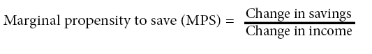
Marginal propensity to save (MPS) refers to the proportion of any extra income that is saved by consumers.
For an individual, the marginal propensity to save will reflect how much they want to put extra income into different forms of saving.
For example, if a worker receives a pay rise of £1,000 and they add an extra £350 to their savings. Their mps will be 0.35.
Marginal propensity to save can also refer to the whole economy. If national income rises £2 bn, and national savings increase £0.1 bn. The marginal propensity to save is 0.05.
Saving function
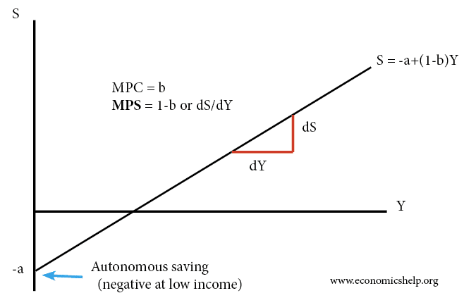
a = autonomous consumption. In this case -a = autonomous saving. At zero income, households borrow to afford the basic necessities of life.
MPS = slope of the savings function. In this case it is -1 + (1-b)Y
How to calculate the MPS
If the change in income = 8% and saving rises 2%. The MPS = 0.25
Why is MPS + MPC always equal to one?
If we ignore taxes and imports, i.e. assume a closed economy. Eith we send money or save it. If we gain an extra £10, and spend £8, by definition the extra £2 is saved.
MPS = 1-MPC
The marginal propensity to save is related to the marginal propensity to consume. Ignoring taxes and imports, the marginal propensity to save (mps) = 1-mpc
Factors that influence the marginal propensity to save MPS
Income levels. At low-income levels, consumers will be buying all the necessities of life. An increase in income, will probably all be spent. At higher income levels, with all necessities bought, saving becomes an affordable extra.
The diminishing marginal utility of income. As income levels rise, extra income has a diminishing utility and so consumers may not know what to spend the money on and therefore spend an increasing percentage.
The Keynesian consumption function shows that the marginal propensity to consume falls at higher incomes – meaning the marginal propensity to save rises.
Life-cycle hypothesis. Theories of life-cycle spending assume individuals wish to smooth out their consumption over a period of time. During a period of studying, marginal propensity to save will be zero (student probably will borrow. As they get a better-paid job and pay off their debts, they will be in a position to increase savings. During their mid-working life, individuals will tend to have a higher propensity to save – as they put money aside for retirement.
Individual preferences. Not all individuals are rational. Approx 25% of individuals do not follow the life-cycle hypothesis models and may fail to save, when rational utility maximisation may suggest they should. Some individuals are more prone to present-income bias. This means individuals place a higher weighting on consumption in present moment, than saving for future.
Risk averse – risk loving. Some individuals are risk-averse, and therefore are more likely to save extra income – planning for unemployment e.t.c. Risk-loving individuals may not wish to save.
Importance of marginal propensity to save
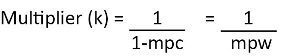
Influences the size of multiplier. A high marginal propensity to save will lead to a smaller multiplier effect. With a high mps, extra income does not ‘trickle down’ to other elements of the economy but gets saved. It reduces the effectiveness of fiscal policy
Marginal propensity to withdraw MPW is the extra income that is withdrawn from the circular flow. Withdrawals = saving, import and tax.
Example
- Suppose the marginal propensity to save = 0.25. In this case, the multiplier is 1/0.25 = 4
- If the marginal propensity to save rises to 0.6. In this case, the multiplier is 1/0.6= 1.66
Related concepts