Time Lags

In economics we often see a delay between an economic action and a consequence. This is known as a time lag.

An impact of time lags is that the effect of policy may be more difficult to quantify because it takes a period of time to actually occur.

Example of time lags

1. Change in interest rate (macro)
2. Increase in level of investment (macro)
3. Change in price of commodity (micro)
4. Effect of devaluation (macro) (J-Curve effect)

1. Interest rate changes

If we cut interest rates, we would expect a rise in investment and consumer spending. This is because lower interest rates make it cheaper to borrow and also make it less attractive to save. Lower interest rates should lead to higher aggregate demand.

However, there may be time lags for a number of reasons.

1. Fixed interest rates for borrowing and saving. Consumers may have a fixed rate mortgage. This means interest payments are fixed for say two years. Therefore, it may be over a year before homeowners actually have to face the higher interest rate.
2. Starting projects. If a firm has started an investment project, they are unlikely to stop just because of an increase in interest rates. Once they have started, they will continue to invest – whatever happens to interest rates. However, over time, the higher interest rates may prevent future investment projects from being undertaken.
3. Knowledge. Consumers don’t have perfect knowledge. They may not check interest rates every month, but only become aware after a certain time.
4. Uncertainty People may wait to see if the interest rate change is temporary or permanent.
5. Bank rates Commercial banks may delay passing on the base rate cut onto consumers.

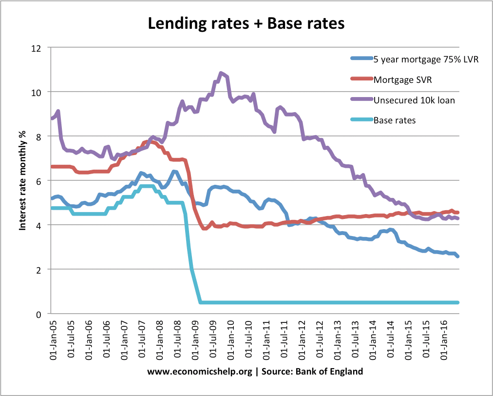
Forward looking monetary policy. Time lags can make policy decisions more difficult. It is estimated interest rate changes take up to 18 months to have the full effect. This means monetary policy needs to try and predict the state of the economy for up to 18 months ahead, but this can be difficult in practise.

Effect of investment

An increase in the level of investment (gross fixed capital formation) will have both short-run and long-run effects.

Investment increases long-run aggregate supply.

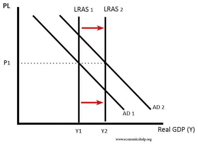
In the short-run, we will see an increase in AD (investment is a component of AD). However, the main effect of investment is an increase in productive capacity. This will lead to an increase in the long-run trend rate of economic growth.

A country which increases the share of GDP devoted to investment may see a fall in consumption in short-run because higher investment requires higher saving. However, in the long-run, the investment can enable increased output and higher living standards.

Time lags and elasticity (micro)

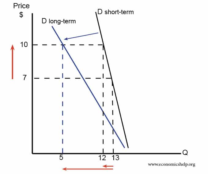
If price rises, then in the short-term, demand is often price inelastic. This is because consumers are in the habit of buying the good and are less aware of alternatives.

However, if the price rise is permanent, they may start to make more effort to look for alternatives. Therefore, over time, demand often becomes more price elastic.

When the price of petrol tripled in the mid-1970s, demand was initially very price inelastic. People with petrol cars still needed to get to work. However, over time, consumers and producers respond to this change in price by developing more fuel efficient cars or even buying an electric car. Over-time, demand has become more price elastic for petrol.

In the short-term a higher price of oil only causes a small fall in demand (13 to 12). However, over time, demand becomes more price elastic and there is a bigger fall in demand.

Short-run, long run and very-long run.

If there is a rise in the price of oil:

• in the short run, demand may be quite inelastic.
• In the long-run, firms can produce more fuel efficient cars and consumers switch to public transport
• In the very long-run, higher oil prices act as an incentive and signal to encourage new technology which diminishes the need for oil, for example, in recent decades, there has been an improvement in the efficiency of solar panels.

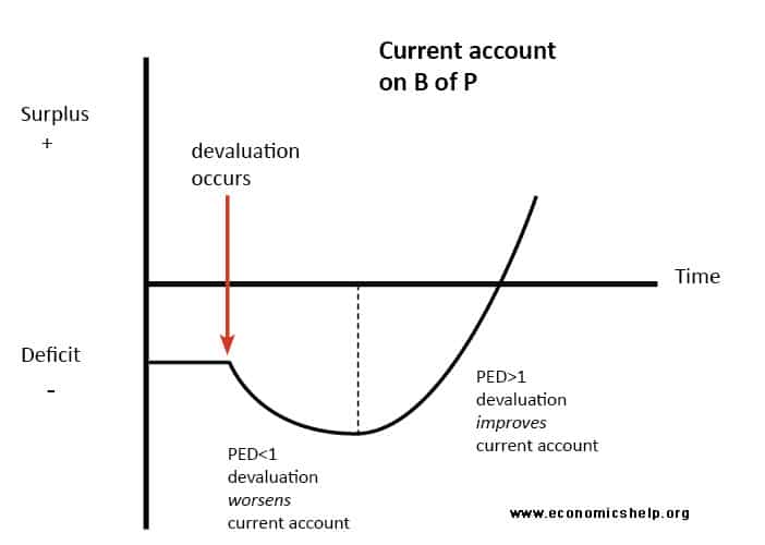
J-Curve effect

The J-Curve effect states that the impact of a devaluation will vary as time progress. A devaluation makes exports cheaper. In the short-term demand is inelastic, therefore, we get a fall in the value of exports and the current account deteriorates.

However, in the long-term, demand for exports is more price elastic, and we get an improvement in the current account.

Irrational exuberance and time lags

It is argued that financial markets can be subject to irrational exuberance. Suppose house prices rise – rising house prices can encourage more people to enter the market to try and benefit from rising house prices. This fuels the rise in house prices even further. Therefore, if we start with a policy of lower interest rates, this causes a rise in house prices, but in the right circumstances, it can lead to a boom in prices. But, at some point the boom comes to an end.

Other examples of time lags

Nearly every issue in economic can be subject to time-lags

For example, if there is a shortage of nurses. This, in theory, should push up wages of nurses. In the very-long run, this may encourage more people to train as a nurse. A shortage of nurses may put pressure on the government to alter its immigration policies.

Related pages

• Effect of increasing interest rates
• Short-run, long-run and very long-run
• Difference between short-run aggregate supply and long-run aggregate supply